Figure 1. Diagram of Harvest Suitability Model.
Geographical (cartographical or spatial) analysis allows you to study real-world processes by developing and applying models. Such models illuminate underlying trends in the spatial data and thus make new information available. In this lab you will create a geographical model using the GIS commands you have learned thus far and the data set from flag24. Read through this entire page prior to starting work on this portion of the assignment.
STEP 1: (Week 7-8) SETTING UP THE MODEL LOGIC
Select 4 to 7 layers to include in a model. Make a flowchart (to turn
in) and design the model. Make a listing of the variables you will include and
take a look at the items (in ArcCatalog), then assign these variables to the classes
suitable or unsuitable (here we have used harvest and no
harvest). Later,
when you write your weighting and classification programs, these two suitability classes will be further
divided into 5 classes: optimal, good, fair, poor, and exclude.
I chose to create a 'Harvest Suitability Model' (courtesy of D.P. Dykstra). We used four layers in this model: Natural Vegetation (pines), Slope, Geology (texture), Streams (200 m buffer).
Figure 1. Diagram of Harvest Suitability Model.
STEP 2. (Weeks 9-10) GET THE DATA
Make sure you copy these data back to your
Z:\ggr525\model folder when you are done
with your editing session, or you will loose all of the edits you have made in
this session!!!
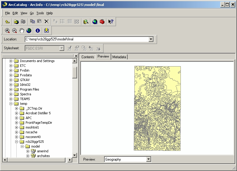
6. Open ArcMap and add the 4 or more layers with which you
will be working. Try displaying several coverages at once in ArcMap, selecting the desired
attributes in each layer. In effect you will see how your model might look before
you actually combine them with overlay commands.
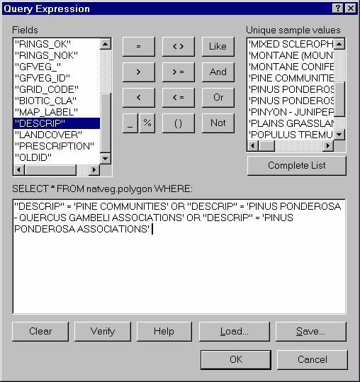
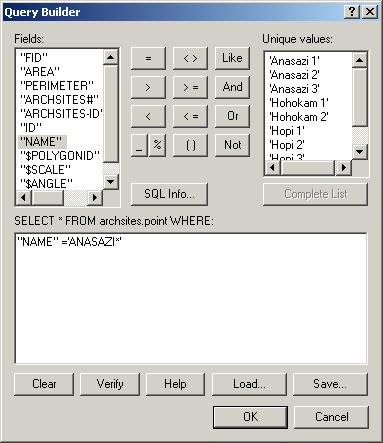
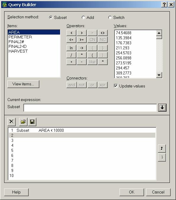
7. For example, say that in our suitability model, we are interested in looking at pine, but not dwarf pines.
So, we construct a query to see just the polygons we want:
STEP 3: (Week 10) PREPARE THE DATA
INTRODUCTORY INFORMATION (yes, read it).
In Exercise 7 you completed a number of buffering processes in ArcToolbox.
Another way to buffer is from ArcMap, but only use ArcMap to test the result of different buffer parameters before committing to one.
You may not want to buffer every feature in a coverage. For example, in archsites, you may want to buffer only Anasazi sites, or only Hohokam sites or both. One way to do this is to:
Name the inside item something unique to that coverage so that when you see it in the final combined attribute table, you will know from where it came.
If you get an error message that stops the buffering process, you may need
to rebuild the topology of your dataset. To do this, open right-mouse click
on the dataset in ArcCatalog, and choose Properties/General/arc/Topology
(Preliminary) /Build.
Also, you will have problems buffering using an item
if the item is named with more than one word. Don't put any spaces in the name,
e.g. use BUFVAL instead of BUFFER VALUE.
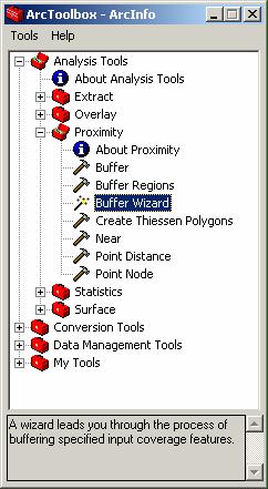
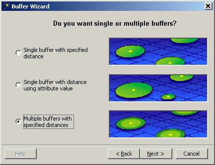
If you want to create multiple buffers of different sizes, use the Buffer
Wizard from ArcToolbox. You can create an interesting buffer using this tool:
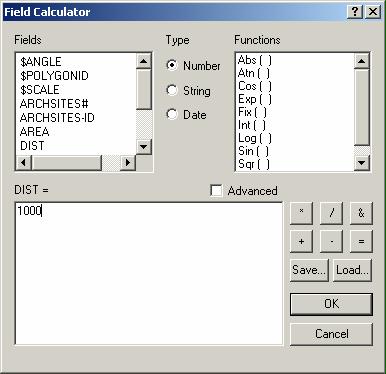
In this case, it is advisable to calculate the inside item values equal to each buffer value:
You can easily change the item name, if necessary, by opening the archsites
dataset
in ArcCatalog, double-clicking point, choosing the Items
tab, highlighting the desired item and choosing Edit.
IF YOU ARE USING MORE THAN ONE BUFFERED COVER (e.g. Roads and Streams),READ THIS NOW (NOT LATER).
Look at the data table for one of your buffered layers. How does the computer know which polygons fall inside the buffer, and which fall outside the buffer? All the polygons are all part of the same layer.
The computer uses an item, or field, either named INSIDE, by default, or whatever you named it when creating the buffers. If you buffer streams and leave the default inside item name (i.e., INSIDE), and buffer roads, leaving the default inside item name (i.e., INSIDE), the inside items of both coverages will have the same name. Eventually, when all the coverages are overlaid, any items with the same name will be dropped from the joining dataset. That means that if you start with strmbuf and add roadbuf to it, roadbuf's inside item WILL BE DROPPED! Hence, THE BUFFERS WILL BE GONE!
To solve this problem, each original dataset that you are buffering needs a unique inside item name, like STRMINSD and ROADINSD.
Make sure all of the layers in your model have the correct codes and explanations in the attribute table; otherwise the information you want to use (which may be in an LUT - look up table - or other file) may be left out and you will have to repeat the overlay process. Therefore, in some coverages you may need to join tables together using ArcToolbox/Data Management Tools/Tables/Join Tables.
Make sure you copy these data back to your Z:\ggr525\model folder when you are done with your editing session, or you will loose all of the edits you have made in this session!!!
CONTINUE EDITING FROM HERE
STEP 4: (Week 10) Combine your model layers using UNION and
IDENTITY.
In this step, you combine all of the layers that will be included
in your model using the UNION and IDENTITY commands. You have used
these commands before.
Note: All of the layers used in this step must
be polygon covers.
Also Note: If you want to use the roads or streams
coverage for reference (not analysis) we will do this later when we plot the
results. Everyone will start with unioning the outerbnd to their
first input coverage.
Here are the steps in general:
...where...XXX is the name of a coverage you have chosen (e.g., landuse, geology, etc.); XXXbuf is a buffered coverage you created in Step 3; overlay1 is the overlay cover resulting from the UNION of two layers, overlay2 is the overlay cover resulting from the UNION of overlay1 and a third cover, etc...
IDENTITY, instead of UNION, is always used with buffered layers so that buffers falling outside the study area are clipped.Do not forget that if you have more than one buffered coverage (e.g., a buffered coverage for streams and another for roads), they will both have an item called INSIDE. You must change the name of the INSIDE items (e.g., STMINSIDE or RDINSIDE) before you overlay them OR one of the INSIDEs will be dropped, removing that buffer from the final cover. Final is the name of the coverage that is a combo of all the layers and will provide your final.pat datafile. Everyone must call this final coverage "final."
Here is a specific example using 3 polygon layers (landuse, slope, geology) and 1 buffered layer (e.g., strmbuf) = 4 overlays in total.
STEP 5: (Week 9) Choose weight values and add your weight item (e.g., HARVEST in my case) to your final
polygon.
When you produce your final polygon layer it will have many fields associated with it from all of the layers
you combined but you will only be interested in certain results. You might be
interested in the Pine Communities of the DESCRIP field, or the 500 value of the
STRMINSD field. You want to summarize the importance of each one of these
variables in a cohesive and understandable way. To do this, you need first
to decide on the importance of each variable via a "weight" between 0
and 10, or -999 if it is excluded from the model altogether. Any
weights you assign to variables must be justified (i.e., results found
in literature, in SCS guide, etc.). You must decide weights in this step (if you
haven't done this previously).
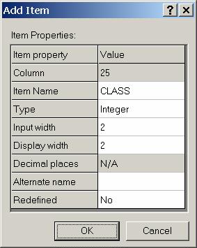
The weights you choose will be held in a new field that you will add to the final coverage (referred to as the weight item). So, add your weight field (e.g., ours was called HARVEST) now, which will hold the results of the weight program run - i.e., all of the weight values added together for each polygon based on each suitability type. Your weight field must be defined as follows (except for the name, which you can change):

STEP 6: (Begin this step during Weeks 9-10; have it completed before Week 12) Write the weighting program.
We will use Visual Basic for Applications (VBA), which is a version of Visual Basic (VB) that runs from inside the application (in this case the application is ArcMap). VB and VBA are part of a suite of object-oriented programming languages. Chris will be talking more about VBA in class.
STEP 7. (Week 12) Run your weighting program.
STEP 8. (Week 12)
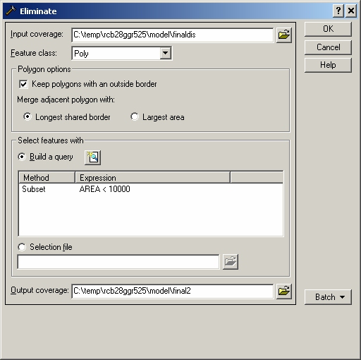
STEP 9: (Week 12) Use ELIMINATE to get rid of those polygons less than the MMU. Everyone will use a ONE HECTARE minimum mapping unit. (Hint: 10,000 sq. meters = 1 hectare). This is to assure that your final plots are not too complex. Look up ELIMINATE in on-line help to learn more.
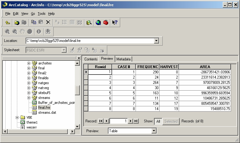
STEP 10: (Week 12) Use the FREQUENCY command to determine the range of values yielded by your weighting program. (Be sure to look for these values in your weight field.)
- From ArcToolbox, double-click the Frequency tool in Analysis Tools/Statistics.
- Use final2 polygon (will appear as final2.pat) as the input table, call the output table final.fre, choose your weight field as the frequency item and AREA as the summary item.
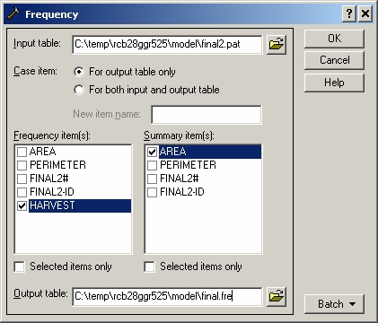
- Select the final.fre file in ArcCatalog to list the results.
C. You can also use the different classification types in the symbol legend in ArcMap (I'll let you figure this out for yourself).
STEP 11. (Week 12 and Week 13...Have your classifying program written prior to class
this week and have it run before Week 13) Add the CLASS field and write the
classification program.
STEP 12: (Week 13...finish before Week 14) Conduct ONE variation of your original model.
This step is the process of generating alternative results. The ideal solution that you attempted last week may not be attainable in practice (which is not uncommon), in which case trade-offs must be made among competing objectives. An iterative process is used to develop alternatives that satisfy these objectives to different degrees or for model "sensitivity" analysis. Of course, we do not have time to develop a whole suite of alternatives, or change every variable to see how "sensitive" the model is to a certain variable, so we will only attempt one iteration.
Conduct at least one variation ("what if") of your model by using a different data layer, enlarging a buffer, and/or changing some variable weights. The more complex your iteration, the more credit you receive. The choice is yours. Be sure to keep track of the output from each change.
STEP 13: (Week 14):
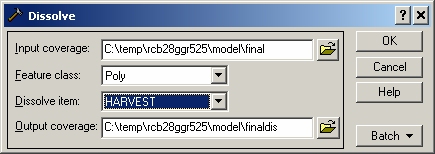
Dissolve your final coverages on the CLASS field. Refer to Step 8 above.
Plot your final products (both the original model and the iteration). The plotting instructions are on the main course page under 'Plotting'.
NOTE: To have the plots print in color, send them to the HP 2500 CM.
STEP 14: (Week 14-15)
Write a summary report of your model. This is due on the last Friday of
the semester before final's week at
4:00 pm. Instructions for page limits, and what to include in your report are
included in the introduction (Time Chart for your Geographical
Model). Turn the whole thing in to your
Lab TA.
STEP 15: (Friday by 4:00 pm, Week 15)
Turn in the model report and have a great winter break!