EXERCISE 7
GIS ANALYSIS: CREATING BUFFER ZONES AND OVERPLOTTING
FOR/GGR 525
BE SURE TO SAVE YOUR WORK REGULARLY!!!
 When
editing a layer in ArcMap, make sure you use the Save Edits option on the Editor
toolbar to save edits as a separate process from saving your map.
When
editing a layer in ArcMap, make sure you use the Save Edits option on the Editor
toolbar to save edits as a separate process from saving your map.
INTRODUCTION
The purpose of this exercise is to introduce the student to another GIS analysis
technique - creating a buffer zone or corridor around features in a coverage.
INSTRUCTIONS FOR COMPLETING THE EXERCISE
Step 1: Formulate criteria for each buffer zone or corridor,
including the specific coverage and its features.
- Coverage = streams (line)
* Generate a 500 m buffer zone on either side of perennial streams over
300 meters in length.
- Coverage = azsoils (polygon)
* Generate a 1000 m, 2000 m, and 3000 m buffer zone around all lithic soils.
- Coverage = aztowns (point)
* Generate differential buffer zones around towns according to their
population sizes.
Step 2: Log-on to the computer, initiate ArcCatalog, and
copy the appropriate coverages (streams, azsoils, aztowns) to your area.
You should have streams in your workspace already.
- In ArcCatalog, connect
 to the flag24/cover folder (See Exercise 1).
- Drag and drop the coverage azsoils to your tutorial folder.
-
Drag and drop the coverage aztowns to your tutorial folder.
- Look at each coverage by previewing the geography and the table.
- Select the look-up tables relating to these coverages (streams.dat and
aztowns.lut) and familiarize yourself with them.
- Be sure you see how aztowns relates to aztowns.lut. Be sure
you see how streams relates to streams.dat.
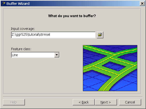
Step 3: Now open ArcToolbox  and select the appropriate line features from the streams coverage,
around which to create a buffer zone.
and select the appropriate line features from the streams coverage,
around which to create a buffer zone.
- In ArcToolbox, click the Analysis Tools plus sign to open the
analysis tools.
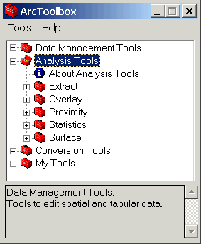
- Click the Extract plus sign.
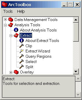
-
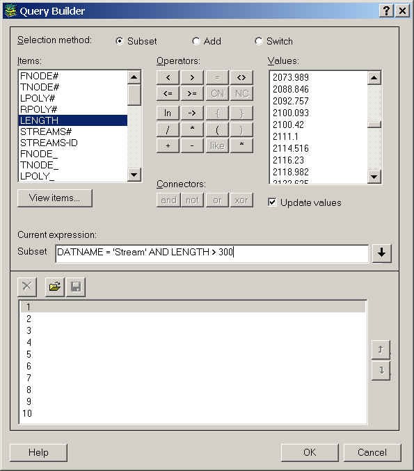
Double-click Select. Select is used to extract map features
from the input coverage based on their attribute values.
-
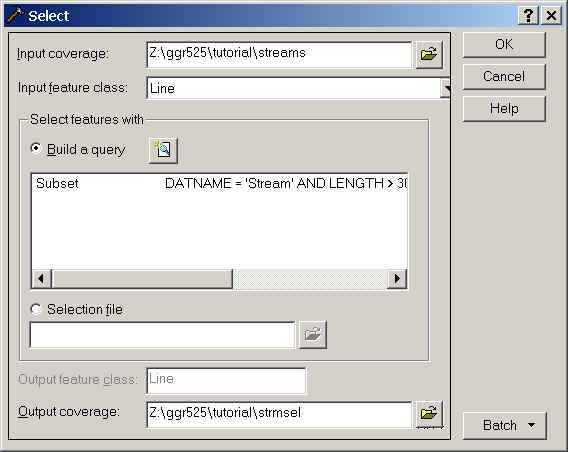
In the Select wizard, enter the streams coverage as the Input
coverage either by browsing for it or dragging and dropping it from ArcCatalog.
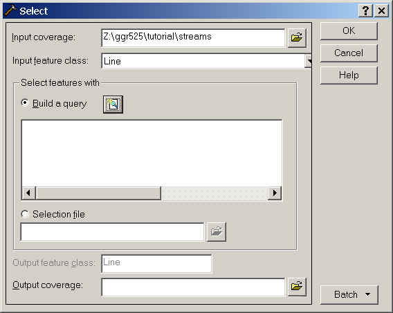
-
Use Build a query to select only those features that are perennial
streams ('stream') and longer than 300 meters.
-
Click DATNAME once.
-
Click the equal sign  .
.
-
Click 'stream.'
-
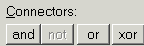
Click the Connector and.
-
Click LENGTH once.
-
Click the greater than sign.
-
Type "300."
-
Click the Add Expression button
 .
.
-
If the expression is valid, it runs and then you can press the OK
button.
-
Name the output cover strmsel and be sure to place it in the tutorial
folder.
-
Click OK.
-
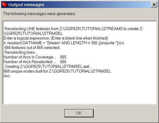
When asked if you want to see the output messages, click OK. The
messages should look something like this:
Step 4: Generate a 500 meter buffer zone around the selected
streams in strmsel according to the criteria for the streams (a line
coverage) coverage and specify an output coverage.
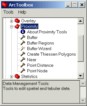
- Go back to ArcToolbox and click the Proximity plus sign.
- Double-click the Buffer Wizard. Read the material presented in each
window as you follow along.
- Choose Output polygons instead of regions and click Next.
- Enter strmsel as the input coverage and click Next.
- Turn on the option of making a buffer at a specified distance. Look
at the other options because you may need one later for you model
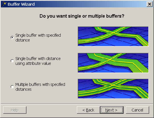
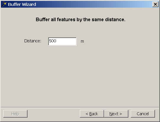
- Enter "500" for distance. The map units are meters since the
coordinate system of our dataset is Universal Transverse Mercator, in meters.
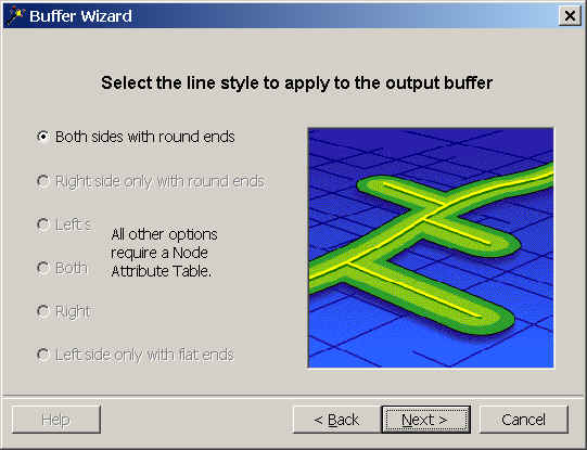
- The buffer style to apply is both sides with round ends. Look at the other
options available in this window for future reference. Click Next.
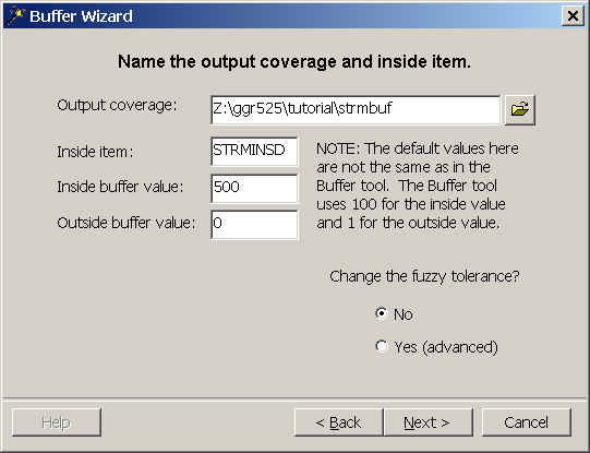
- Name the output coverage strmbuf, make the item which holds the value of
inside or outside strminsd, and make the value for areas inside the
buffer zone "500." Click Next.
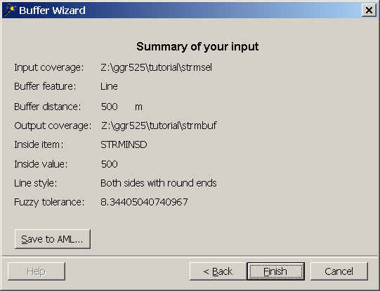
- ArcToolbox tells you what it's about to do for verification. Click Finish if the parameters are correct.
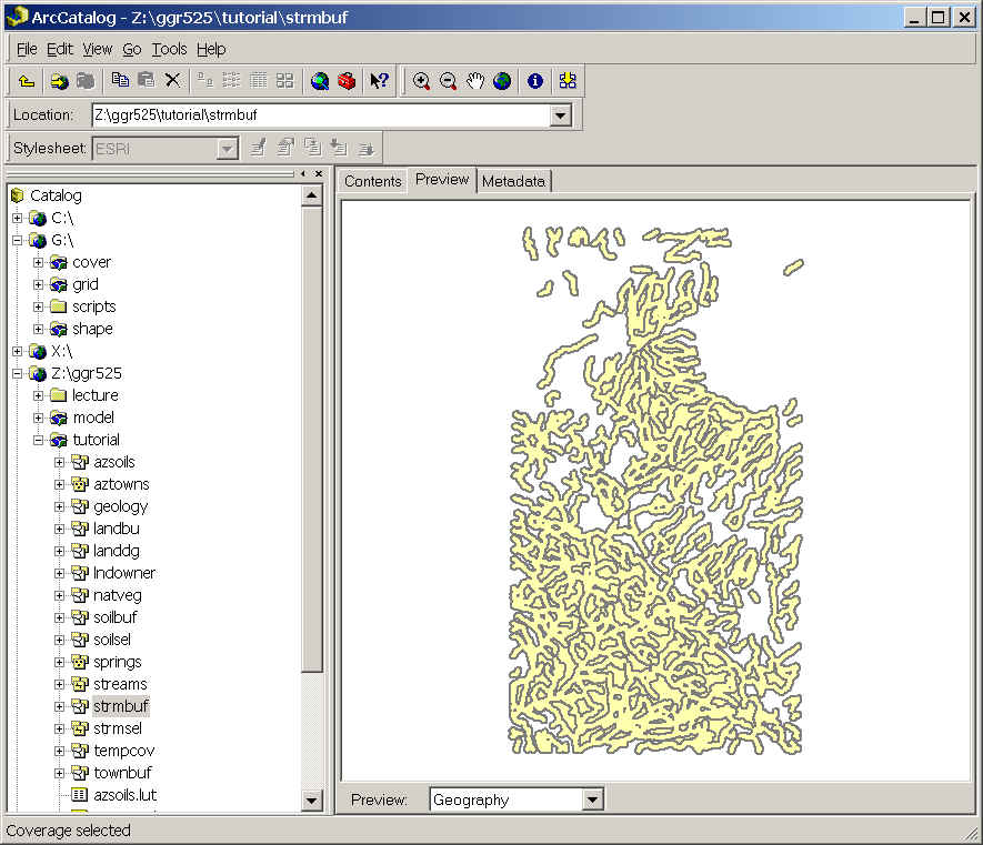
- Preview strmbuf in ArcCatalog to be sure the buffer function
worked properly.
Step 5: Repeat Steps 3) and 4) for the second coverage.
- Select the lithic soils from azsoils.
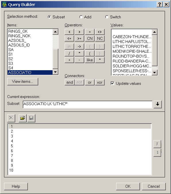
- Go back to ArcToolbox/Extract/Select.
- In the Query Builder use Like and the wildcard (*) to
find all soils containing the word "LITHIC."
- Name the output soilsel.
- Be sure to look at the messages. You should have extracted 2 polygons
out of 15.
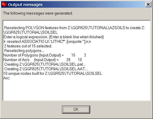
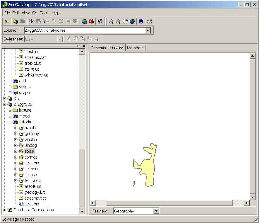
- Look at the output polygons by previewing soilsel in ArcCatalog.
Buffer soilsel with 3 rings of 1000, 2000, and 3000 m
consecutively.
- Go back to ArcToolbox/Analysis Tools/Proximity/Buffer Wizard.
- Choose Output polygons. The input coverage is soilsel and the feature class is poly.
- The type of buffer is "multiple buffers with specified distances."
- Choose "3" rings and enter the proper values. The buffers are
drawn for you. Notice that you could make rings bigger or larger as you move
away from the target.

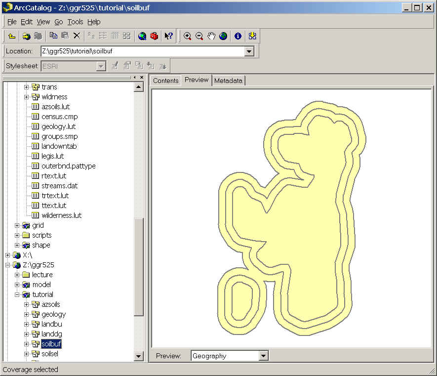
- Name the output soilbuf and choose appropriate names and values.
Click Next.
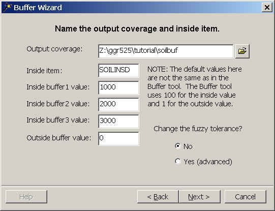
- In the Summary of your input window, check the settings and then click Finish.
- Preview the geography of soilbuf in ArcCatalog.
Step 6: Add buffer distance values to a lookup table for differential buffer zones
around aztowns that have varying populations.
- Look at aztowns.lut in ArcCatalog. It has a population
field, but we don't want to use these values to buffer since each will be a
different size, and there will be a large dichotomy between buffer sizes.
- So, we will add a buffer distance value for different populations. Use the following criteria for differential buffer
zones in the following steps.
| POPULATION |
BUFFER DISTANCE (m) |
| < 100 |
1000 |
| 100 - 999 |
2000 |
| 1000 - 10000 |
4000 |
| > 10000 |
8000 |
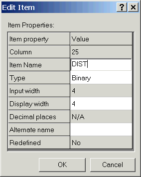
- Add an item (field) to aztowns.lut to hold the buffer
distance values.
- In ArcCatalog right mouse-click aztowns.lut and choose Properties.
- Click the Items tab.
- Click the Add button.
- Enter the following Item Properties values. As we will only
need 4 display digits, we can use "binary," which takes less
space (2 bytes per character) than do 4 integer digits (which take 8
bytes per character). Be sure to name the new item "DIST."
-
Open ArcMap, and use the Add Data button to add aztowns
point and aztowns.lut to a new map. If you get a message about
the layer missing spatial reference information, you can add this to your
data in ArcCatalog (see Exercise 2 for procedure).
-
Select aztowns point, open the Editor Toolbar
and choose Editor/Start Editing.
-
Right mouse-click aztowns.lut in the Source
window and choose Open.
-
Click in each cell and enter the proper distance based on
the table above.
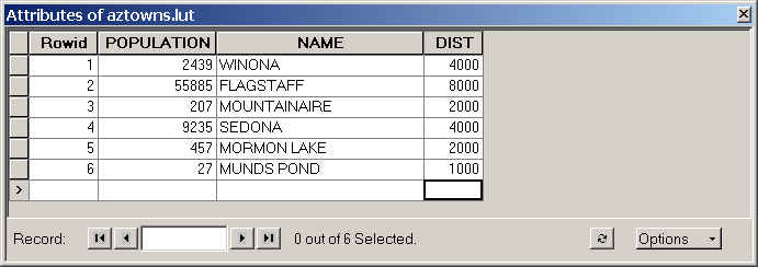
-
Save your edits with Editor/Save Edits.
-
If you had many more values, you would copy aztowns.lut
to make a new table with a different name, and enter a range of values for
the population and corresponding buffer distances.
-
You can also make a new table using INFO or from ArcToolbox/Data
Management Tools/Tables/Define Table.
Step 7: Repeat Steps 3) and 4) for the third (aztowns) coverage;
however, you need to use the aztowns.lut table.
- From ArcToolbox, start the buffer wizard.
- Choose Output polygons and perform a buffer at a distance from an attribute.
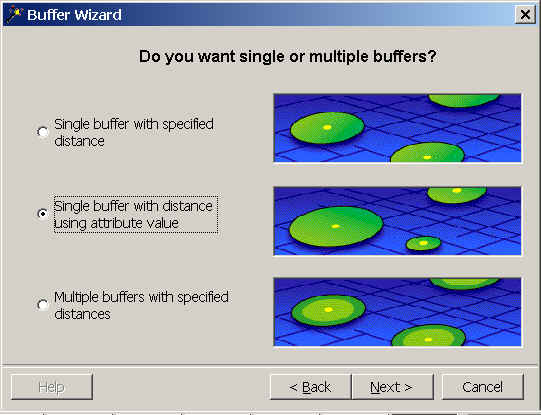
- Before choosing the distance item, check the Use a look up table for the item
values option and browse for aztowns.lut.
- Be sure the Distance item is "NAME."
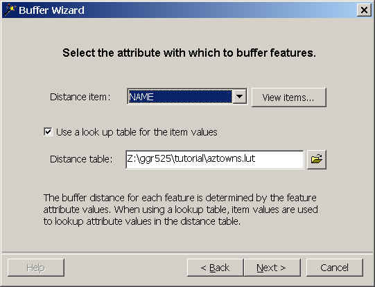
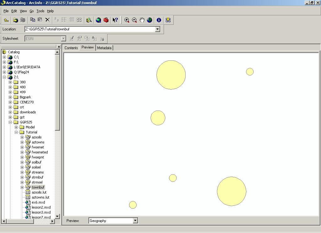
- Name the output townbuf, and the output buffer item TOWNINSD.
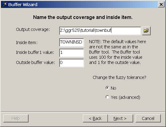
- Look at townbuf in ArcCatalog to make sure the buffer
process worked correctly.
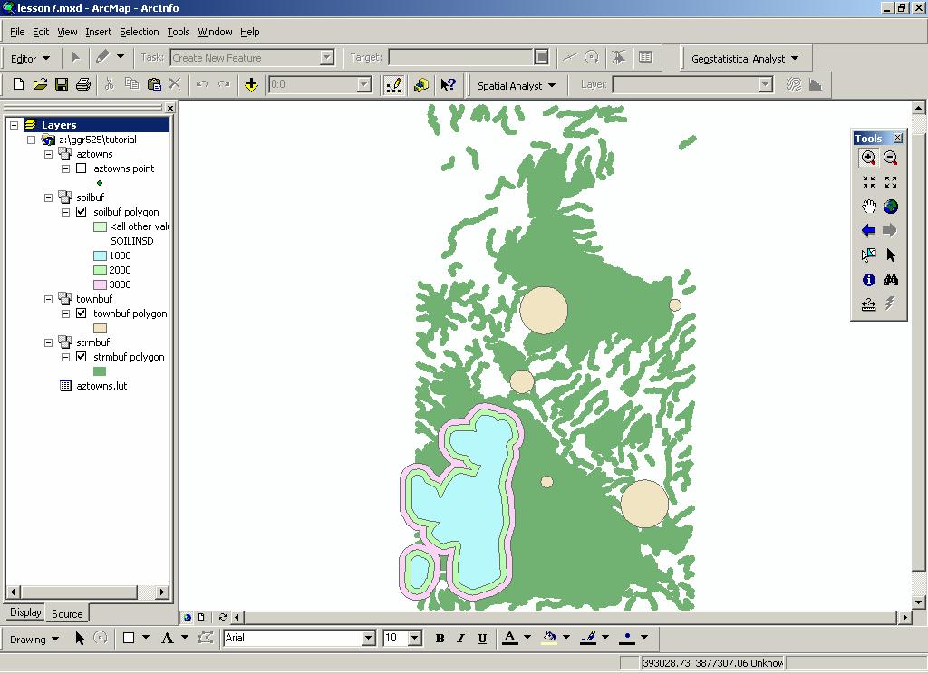
Step 8: Display the output coverages together and evaluate the results.
Before you do this, however, you should be aware of some basic differences
between combining coverages for display (this exercise) and combining coverages
for analysis (Exercise 8). For the purpose of displaying information, individuals
layers do not have to be combined. A composite display of their individual
features can be obtained by plotting several coverages on top of one another
(Step 8c). This technique is known as OVERPLOTTING. You will use this technique
again later with your MODEL exercise so that you can see the implied
relationships before you actually combine the coverages.
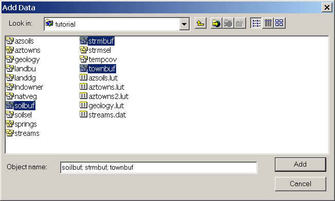
- Open ArcMap.
- Click the Add Layer button and add strmbuf, townbuf, and
soilbuf . Use the Ctrl key to select all three coverages.
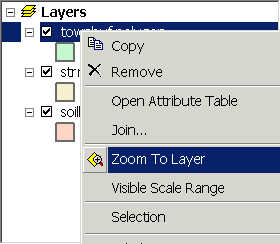
- Right mouse-click townbuf polygon and choose Zoom to Layer.
- In the Display view of the Table of Contents, select the soilbuf polygon layer and drag it above strmbuf
polygon so that the soils draw on top of the streams. If your layers
drew this way automatically, skip this step.
- Draw the soilbuf buffers using different colors.
- Double-click soilbuf polygon and choose the Symbology tab.
- In the Show window show Catagories: "Unique
Values."
- For Value Field select "SOILINSD" and click the Add
All Values button.
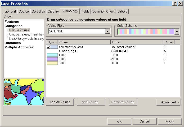
- Click OK.
- Now you can see how different buffers overlay other polygons.
- Make a layout showing the combinbed stream, soils, and town buffers,
and hand it in to your TA.
In the next exercise we will
physically overlay (combine) coverages.
 Return to Class Home Page...